Large 3D Data

Motivation
Start with the bottleneck: what is too large?
Too large for what
- Disk
- RAM
- Graphics memory (VRAM)
- The network
Approaches
- Layout - optimize how the data is stored
- Streaming - optimize access to the data
- A cheaper representation - reduce the amount of data itself
Data Layout optimization
Structuring Volumes
Data Layout optimization
Structuring Volumes
Support chunks & multiple resolutions
- In one file:
- HDF5
- OME-TIFF
- In a multi-file structure:
- OME-Zarr
- N5
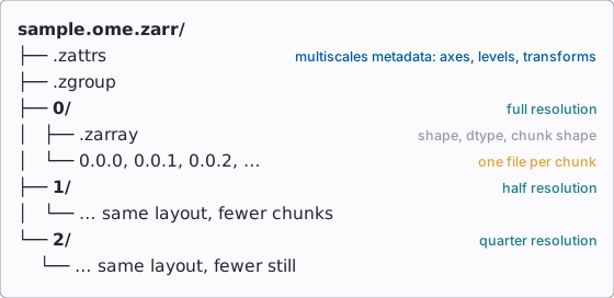
OME-Zarr file tree
Data Layout optimization
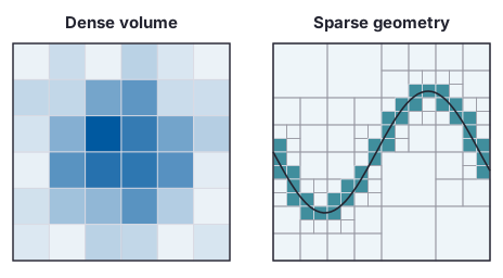
From dense volumes to sparse 3D data
Dense volume
- Data fill the grid
- Regular chunks work well
- Same structure at every location
Sparse geometry
- Data occupy only part of space
- A fine grid would contain many empty cells
- Use spatial subdivision instead
Data Layout optimization
Sparse geometry
Octree
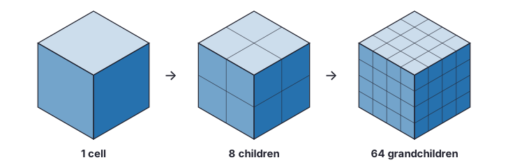
One cell, subdivided into eight children, each subdivided again into eight grandchildren of its own.
- Empty regions stay coarse
- Data-rich regions become fine
- Depth gives a natural level of detail
- Armadillo: Stanford 3D Scanning Repository, courtesy of Helmut Kungl, non-commercial/educational use with credit · preparation script
Data Layout optimization
Spatial hierarchies make large geometry scalable
Point clouds
- Organize points spatially
- Load/refine only visible regions
- COPC, EPT, Potree
Surface meshes
- Organize geometry in spatial patches
- Stream appropriate levels of detail
- 3D Tiles, Nexus
Adaptive simulation meshes
- Hierarchy defines computational cells
- Refine only where needed
- t8code
Visualization based on optimized layouts
Example: BigVolumeViewer
- GPU cache of blocks
- Block = chunk at one resolution level
- Pietzsch, Saalfeld, Preibisch & Tomancak (2015), BigDataViewer: visualization and processing for large image data sets
Visualization based on optimized layouts
Example: PoTree
- Point budget: maximum points per frame
- Descend into whatever looks biggest on screen, until the budget is spent
- What gets drawn is a cut through the tree - deep near the camera, shallow far away
- Canyon: USGS 3DEP, public domain, via the AWS Open Data Entwine mirror · preparation and octree build · vertical relief exaggerated 3x · Potree · Schütz (2016), TU Wien
Streaming
Goal: share a large dataset without sending the whole dataset
- Convert once → chunked, multi-resolution data
- Host somewhere, share a URL
- Viewer fetches only what the current view needs
Local vs. remote
- Localhost → only you
- Temporal server via HPC node IP → stream from HPC to local visualization tool
- Public host → anyone with the URL
- Viewer receives a data address
Streaming
Examples of links including both the data and the viewer
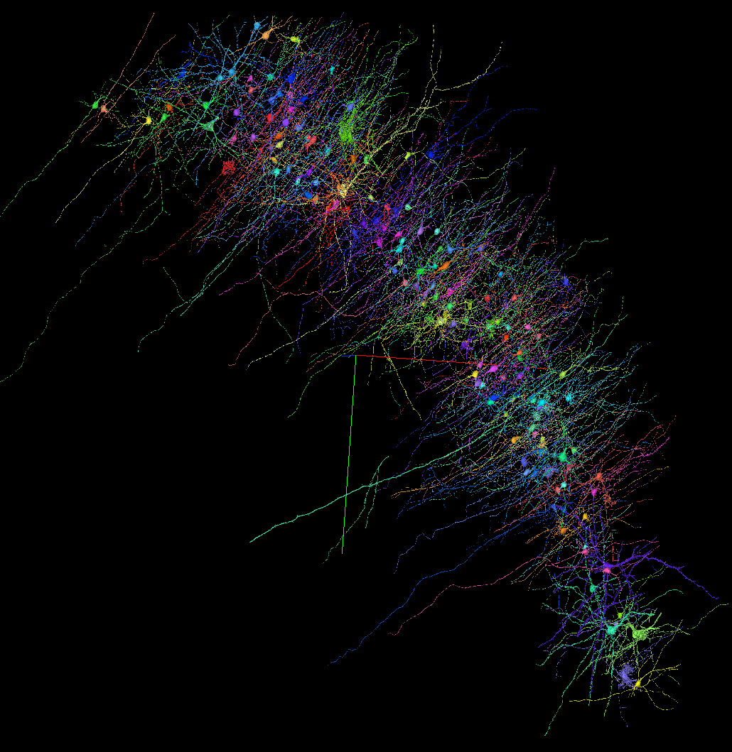
Neuroglancer · 1.4 PB of human cortex
H01 · Shapson-Coe et al. (2024), Science 384
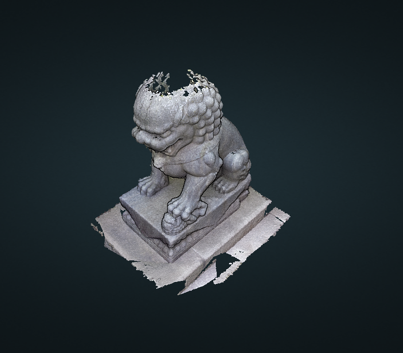
Potree · a laser-scanned stone lion
Potree, from its own example set
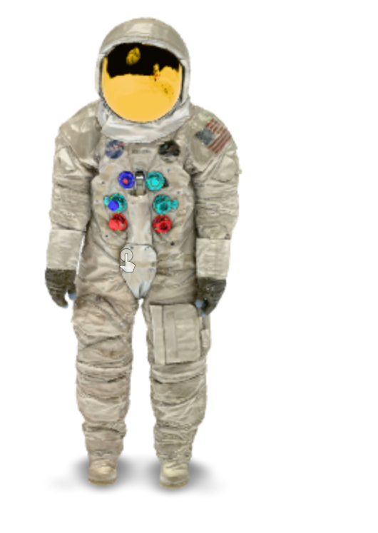
<model-viewer> · one glTF on a page
Spacesuit: Smithsonian Digitization Program Office
Streaming
What a viewer needs from the server
- Static host → serves files
- Browser → renders data
- CORS → permits cross-origin requests
- Byte ranges → permits partial file requests
access-control-allow-origin(CORS) - a browser reads a file from another host only when the response carries it. Without itcurlworks and the viewer stays emptyaccept-ranges: bytes- lets a viewer ask for part of a file. Needed by COPC, zipped Zarr and Potree’soctree.bin- Check headers with
curl -I:
curl -I https://your-host.org/my-dataset.ome.zarr/.zattrs
Streaming
Where to put the data
- dCache / InfiniteSpace at DESY, through HIFIS - no size limit, can be public
- S3 or Google Cloud Storage - set the bucket’s CORS policy
- BioImage Archive - for published data
- Your own machine -
python server.py -d <dir>, port 8082, CORS open
- HIFIS dCache documentation · hifis-storage.desy.de ·
server.py, from the Neuroglancer repository
Compact scene representations
Borrowing from Computer Vision
- Developed for computer vision
- Classical input: photographs of a real scene, and where each camera stood
- Goal: realistic looking reconstruction of the 3D environment
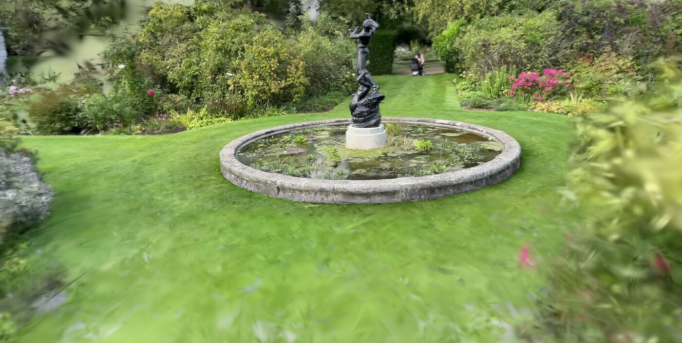
A garden captured on a phone and fitted as Gaussian splats. Credit: Óscar Mirás on Wikimedia Commons, CC BY-SA 4.0

Compact scene representations
NeRFs
Implicit representation
- Scene = learned function
- Query any position in space → density + appearance
- Sample repeatedly along a camera ray
- Volume-render the samples
Think of it as: volume rendering, but query a trained function instead of reading a voxel.
- NeRF: Mildenhall et al. (2020), Representing Scenes as Neural Radiance Fields for View Synthesis, ECCV · figure script
Compact scene representations
3D Gaussian Splatting
Explicit representation
- Scene = 3D Gaussian primitives
- Project them onto the screen → 2D elliptical splats
- Sort + alpha-blend
- Render directly
- 3D Gaussian Splatting: Kerbl et al. (2023), 3D Gaussian Splatting for Real-Time Radiance Field Rendering, SIGGRAPH · figure script
Compact scene representations
Example of a Gaussian Splat fit
- Target: A crop of a micro-CT scan of a sunflower head. Chitwood, Quigley & Frank, X-ray CT Botanical Images - Set 1, Zenodo (2025), CC BY 4.0
- Fitting and rendering: luxar · fitting script
Tools
Voxels: Convert and validate
- Workshop notebook: tiff_to_ngff_and_neuroglancer.ipynb - TIFF → pyramid → validate → serve → Neuroglancer
- Vendor formats → bioformats2raw
- NumPy → ngff-zarr / ome-zarr-py
- Fiji → MoBIE
- Multi-tile acquisitions → BigStitcher
- Check the result → OME-NGFF validator
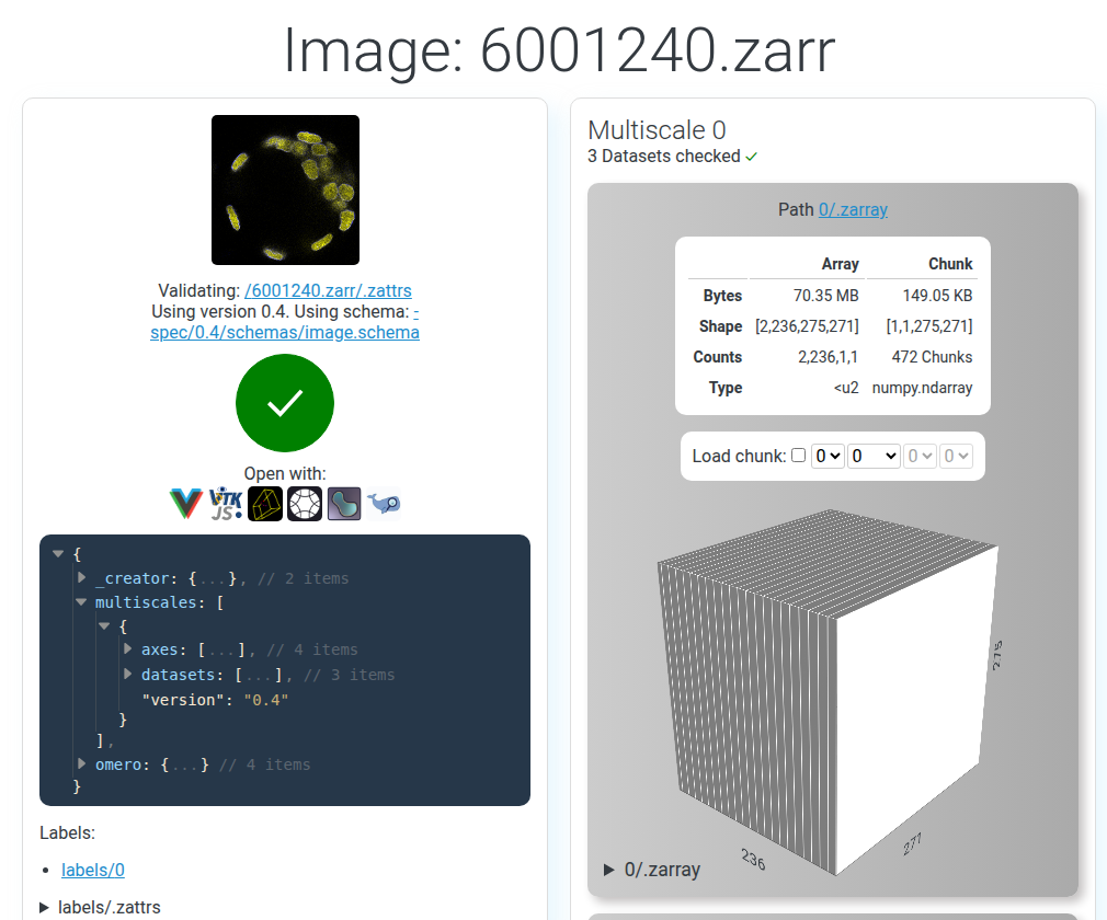
The OME-NGFF validator checks the OME-ZARR structure.
Tools
Voxels: View and work with the same pyramid
Local / desktop
- BigVolumeBrowser / MoBIE → GPU volume rendering
- napari → general Python-based exploration
- 3D Slicer → clinical and biomedical volumes, segmentation, registration
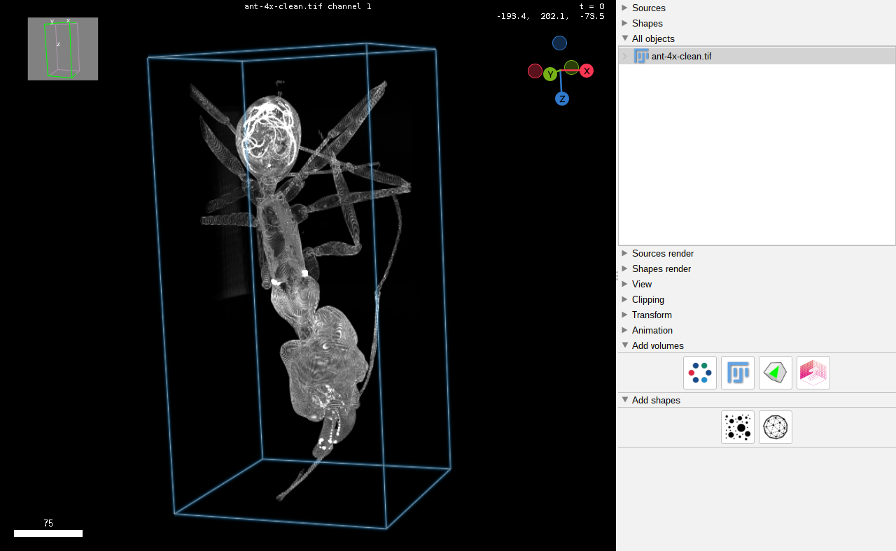
BigVolumeBrowser rendering a synchrotron scan of a trap-jaw ant.
- Ant: synchrotron micro-CT from Antscan, a digital library of 3D invertebrate anatomy by Katzke, van de Kamp & Economo · Katzke et al. (2026), High-throughput phenomics of global ant biodiversity, Nat Methods 23, 663–672 · scans via BIOMEDISA and RADAR4KIT
Tools
Voxels: View and work with the same pyramid
Browser / sharing
- Neuroglancer → volumes + segmentations
- webKnossos → collaborative annotation
- Viv → multiplexed microscopy
Work on the data
Tools
Point clouds: Convert once, then stream the hierarchy
- Covered in the point clouds session, with the commands to run
- PDAL → read and write about anything, and reproject it
- PotreeConverter / Entwine → build the hierarchy
- Potree → browser visualization
- CloudCompare → desktop exploration, cleaning, alignment
- COPC → the same octree in one LAZ file
Tools
Meshes: Reduce, compress, or stream
Prepare
View
- Nexus → large multi-resolution meshes
- Blender → desktop inspection + editing
<model-viewer>→ glTF in the browser
Tools
Voxels or points → Gaussian splats with luxar
- Workshop notebook: luxar_gaussian_splats.ipynb - install, compile, fit, serve
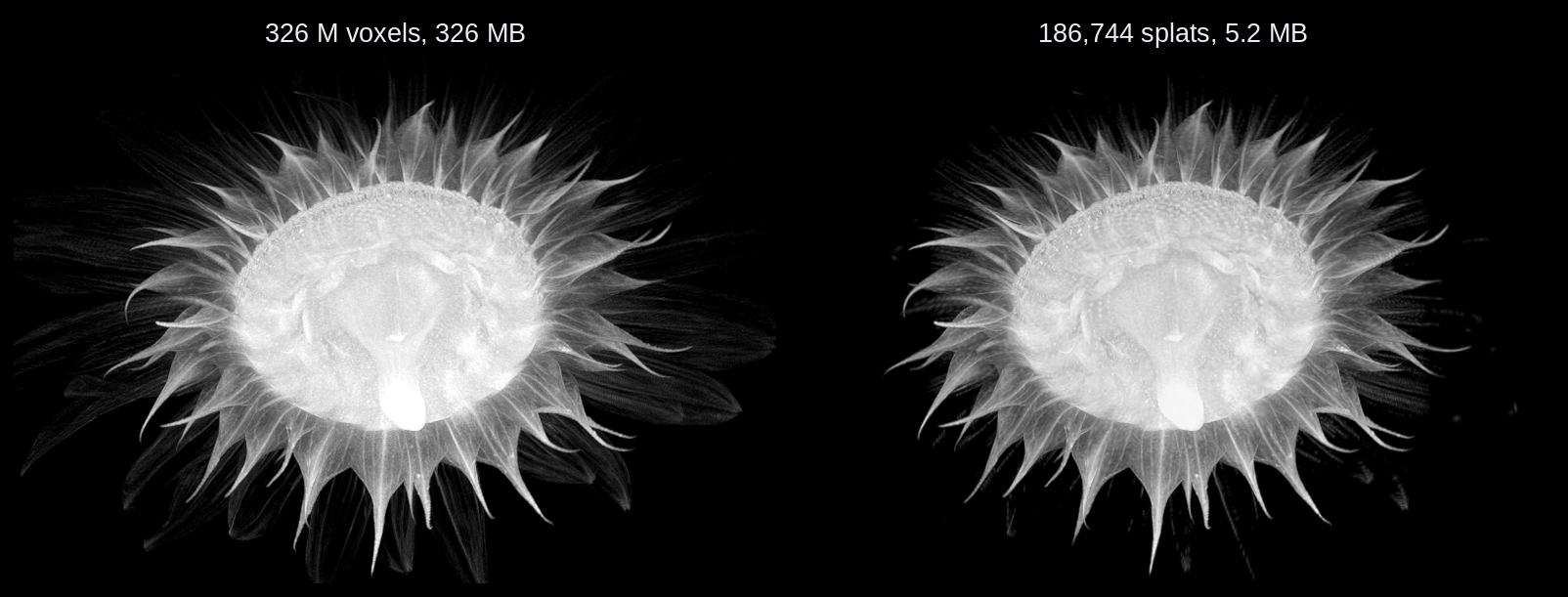
The micro-CT volume and its fitted Gaussian-splat representation.
- Sunflower: Chitwood, Quigley & Frank, X-ray CT Botanical Images - Set 1, Zenodo (2025), CC BY 4.0