3D Data Visualization Workshop
Deborah Schmidt
Head of Helmholtz Imaging Support Unit, MDC Berlin
Sep 17, 2025
3D Dataset types
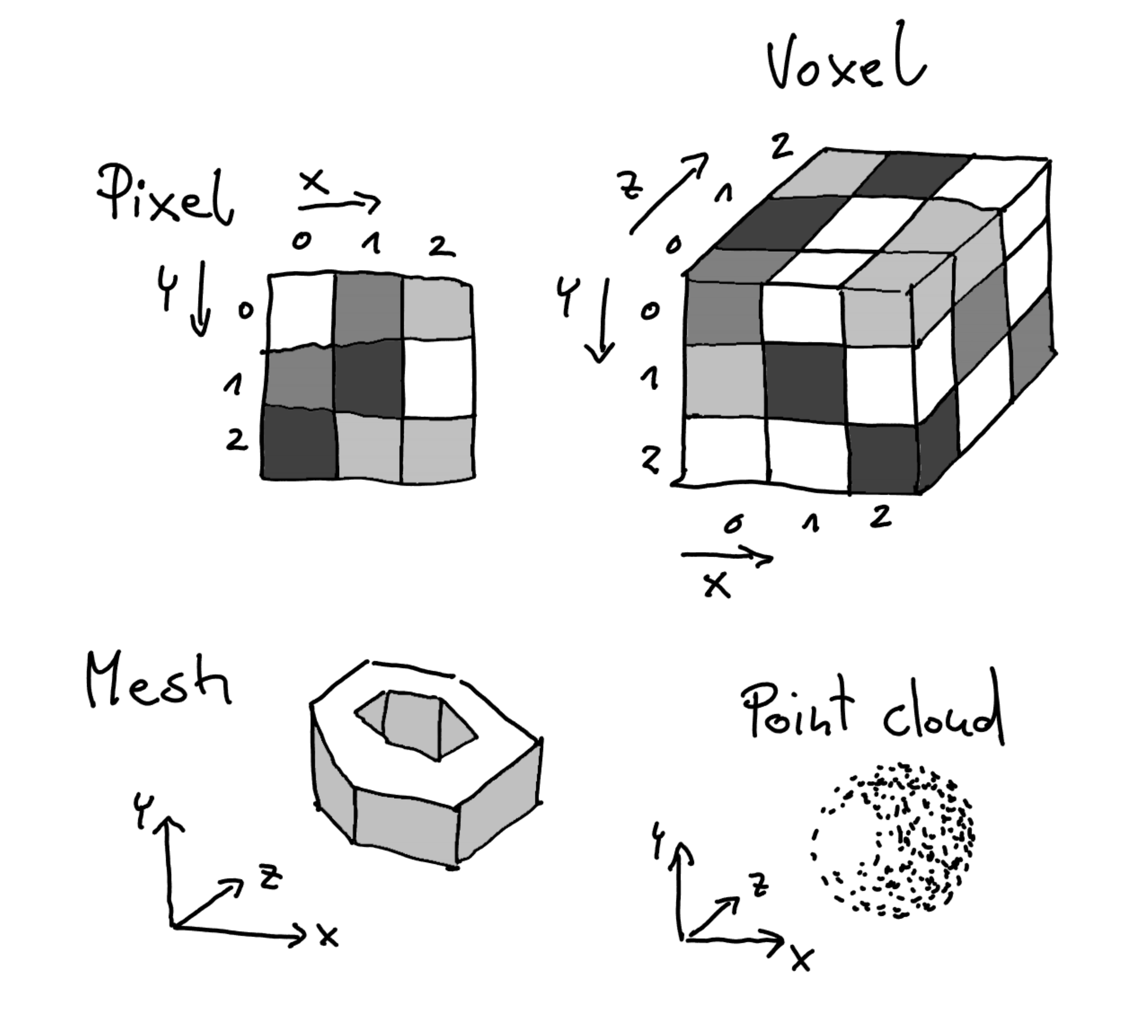
- Voxel-Based Datasets (Euclidean-structured)
- Meshes (Non-Euclidean-structured)
- Point Clouds (Non-Euclidean-structured)
- Vector Fields (structured or unstructured)
Voxel‑Based Images
- What is it? 3D grid (voxels) with scalar (or vector/tensor) values.
- Acquire (by domain): CT/MRI, light‑sheet/confocal, micro‑CT, simulations.
- Used for: Inspect interiors, segment/analyze regions, measure volumes.
- Stored as: TIFF stacks, NIfTI/NRRD, HDF5, OME‑Zarr (great for big data & web).
- Visualized with: Orthogonal slices, volume ray casting, MIP, isosurfaces.
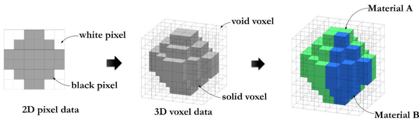
Voxel based data representation. Credit: Hasanov, S. et al. (2021), CC BY-SA 4.0.
Voxel‑Based Images
Voxel spacing, anisotropy
- Spacing = physical size per voxel (e.g., 0.2 × 0.2 × 1.0 µm).
- Isotropic: spacing equal along axes → cubes; anisotropic: one axis differs (common in microscopy & clinical CT).
- Always set spacing in your viewer/exporter.
- In napari, set “Scale” in layer properties.
- In VTK/ParaView, set “Data Spacing” or use image origin/spacing fields.
- Resample if needed (trade speed vs fidelity): upsample Z for nicer isosurfaces; downsample big XY for faster previews.
Voxel‑Based Images
Visualizing volumetric datasets
- Slice‑based: axial/sagittal/coronal (medical) or arbitrary oblique slices.
- Maximum/Minimum Intensity Projections (MIP/MinIP): great for vessels or bright structures.
- Emission‑absorption (volume ray casting): assign color + opacity by intensity (“transfer function”); can add lighting.
- Isosurface: fast surface extraction at a threshold (marching cubes) for clean boundaries.
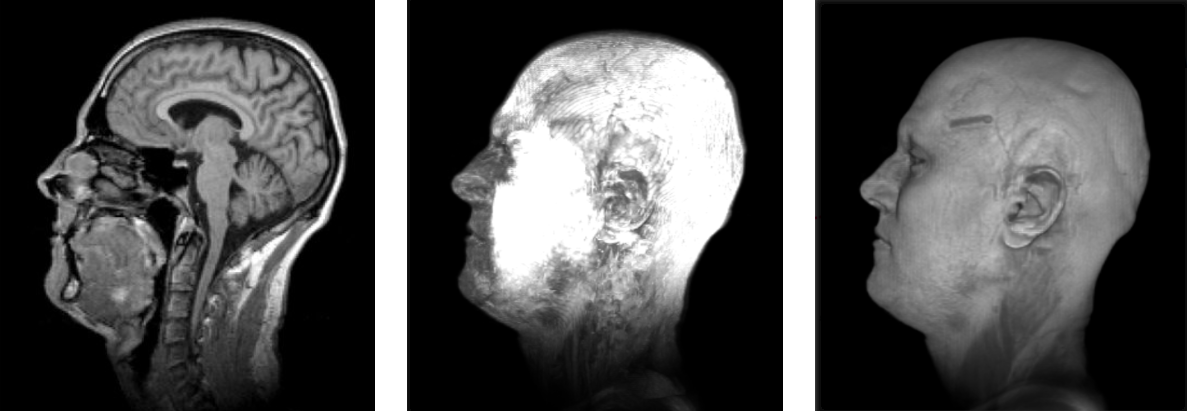
Slicing, Max. Intensity, Emission Absorbtion

Voxel‑Based Images
Volume Rendering in napari
- Interactive visualization and annotation: Offers tools for exploring data and annotating images in real-time.
- Layer-based rendering: Supports multiple layers like images, labels, points, and shapes for versatile data representation.
- Plugin extensibility: Easily extendable through plugins to add custom functionality.
- Integration with Python ecosystem: Seamlessly works with NumPy, Dask, and other scientific Python libraries.
Voxel‑Based Images
Praxis: Visualizing volumes with napari
- Open napari → File → Open… a 3D stack (TIFF/OME‑TIFF/NIfTI/Zarr).
- In the Layers panel, select your image layer:
- Set Scale to the correct voxel spacing (e.g.,
0.2, 0.2, 1.0). - Switch 2D → 3D (bottom left bar).
- In Rendering, try: MIP, Translucent/Attenuated, Iso.
- Set Scale to the correct voxel spacing (e.g.,
- Adjust the contrast limits and colormap; add a labels layer if you have a segmentation.
- File → Save Screenshot to export a figure (optionally with a transparent background).
Photogrammetry

Jan-Simon Schmidt (HZB), Ole Johannsen (DKFZ, Helmholtz Imaging), Deborah Schmidt (MDC, Helmholtz Imaging)
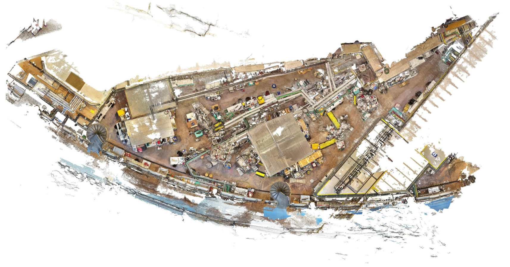
Photogrammetry
- What is it? Recover camera poses (SfM) → compute depth (MVS) → output dense point cloud and mesh+texture.
- Acquire (by domain): Drone surveys, cultural heritage, lab setups; consistent overlap & fixed focal preferred.
- Used for: Reconstruction, measurement, communication, web sharing.
- Stored as: Images + camera models, PLY/OBJ/GLB mesh, LAS/PLY point cloud, optional orthomosaics/DEMs.
- Visualized with: Mesh or point‑based viewers; geospatial tools when georeferenced.
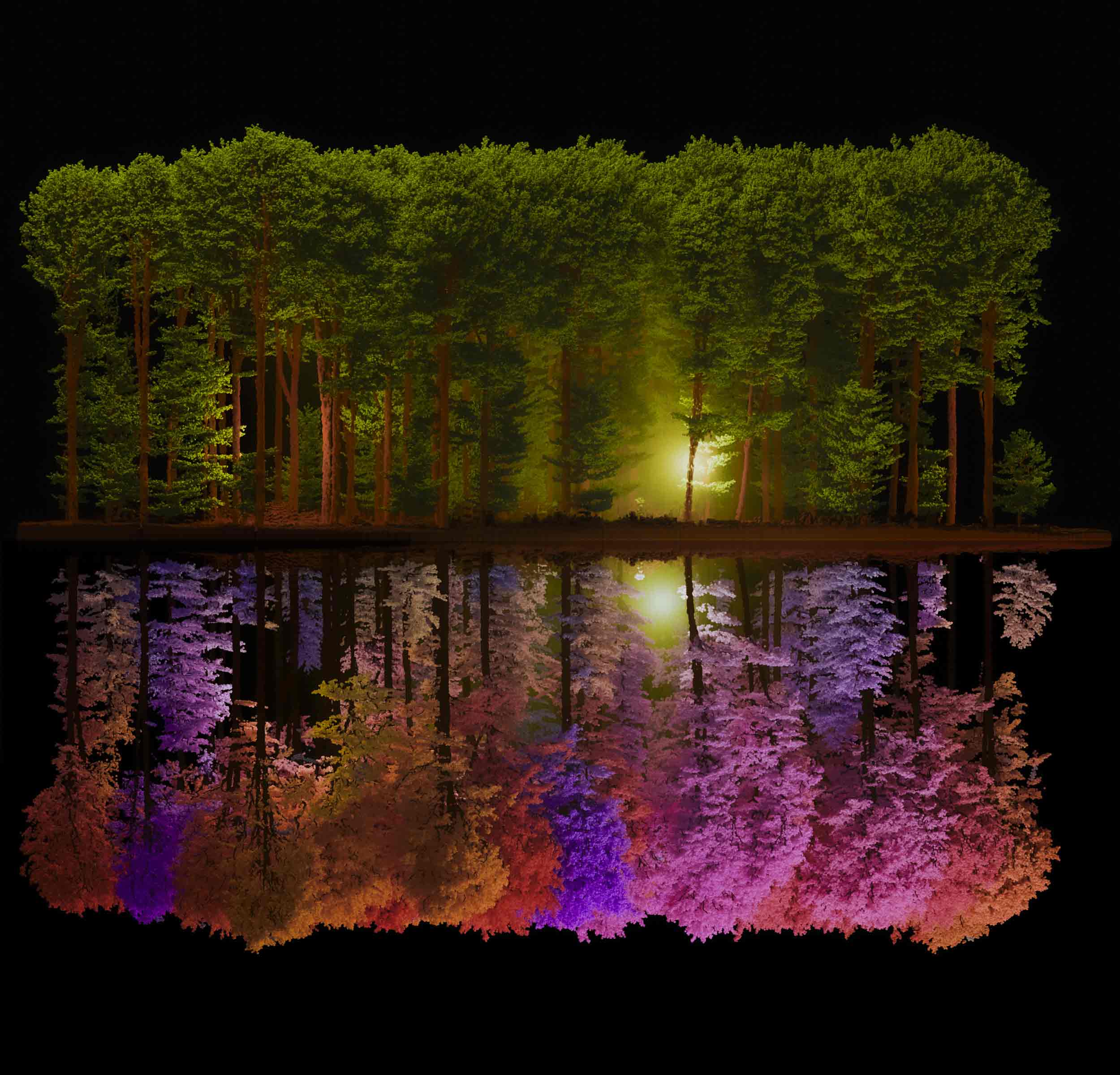
Point clouds
- What is it? A set of 3D points with attributes (intensity, color, class, time…).
- Acquire (by domain):
- LiDAR (ground/airborne), depth sensors.
- Photogrammetry (dense matching).
- Microscopy (particle centers, single‑molecule localizations).
- Used for: Mapping, fitting, statistics, reconstruction.
- Stored as: LAS/LAZ, E57, PLY, CSV/Parquet; for the web: EPT (Entwine Point Tiles).
- Visualized with: Point rendering (“Point Gaussian”), color by attribute, subsampling & LODs.
Point clouds
Rendering challenges
- No connectivity → consider surface reconstruction (e.g., Poisson, alpha‑shapes) when needed.
- Often noisy & redundant → filter, align, downsample, and normalize intensities.
Point Clouds
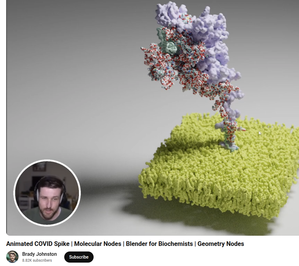
Domain-Specific Variants
- Many scientific domains represent data as points in 3D space with domain-specific attributes.
- Atoms in molecules → standardized formats (PDB, mmCIF), rendered as spheres/bonds
- Stars in astronomy → catalogs (FITS, VOTable), rendered as brightness-colored points
- Cells in microscopy → tables or SWC/OME formats, rendered as centroids or markers
- Same principles apply, but with tailored formats & rendering techniques
Point clouds
Praxis: Visualizing point clouds with ParaView
File → Open… a LAS/LAZ/PLY or CSV with XYZ.
Click Apply. In the Properties panel:
- Set Representation = Point Gaussian for smooth points.
- Increase Gaussian Radius until points visually connect.
Point clouds
Praxis: Visualizing point clouds with ParaView
Add filters as needed (Filters → Search):
- Clip (box/plane) to isolate a region.
- Decimate (Points) or Mask Points to downsample for speed.
Save a screenshot or File → Export Scene for vector graphics.
Meshes
- What is it? Vertices + faces define a continuous surface.
- Acquire (by domain): From segmentation (marching cubes), CAD, photogrammetry, simulation output.
- Used for: Visualization, 3D printing, analysis (curvature/area), animation.
- Stored as: STL, PLY, OBJ, GLB/GLTF, VTP; textures as PNG/JPEG; materials in MTL/GLTF.
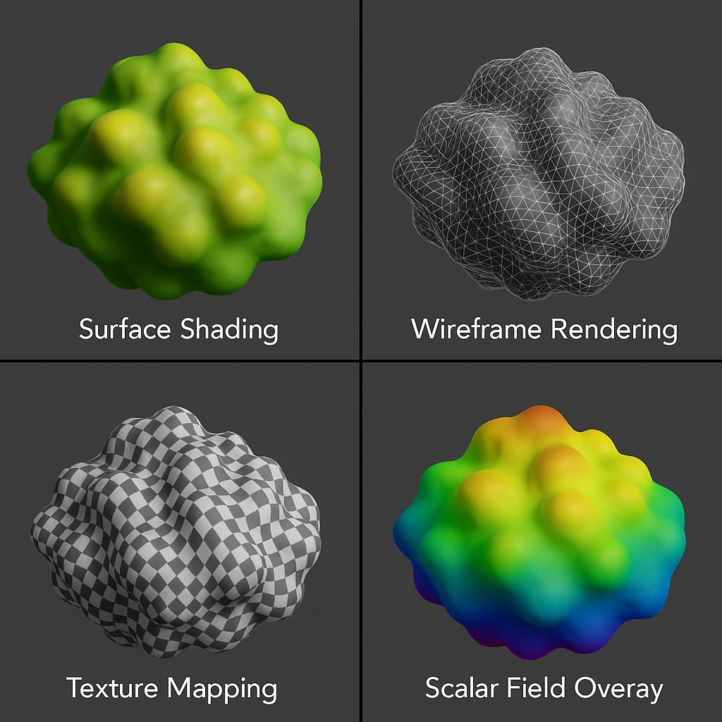
- Visualized with: Smooth shading, PBR materials (Physically-Based Rendering, for textured assets), scalar maps, cuts/slices.
Mesh processing
Tools
MeshLab: A powerful tool for cleaning, decimating, and refining 3D meshes. It supports:
- Smoothing: Remove sharp edges or rough areas in the mesh.
- Decimation: Reduce the number of polygons while maintaining the overall shape.
- Repair: Fix holes or non-manifold geometry in the mesh for better usability.
Other tools: Blender and VTK also offer additional mesh processing capabilities.
Rendering meshes
Meshes
Rendering pipeline
- Vertex shader: places points in the scene.
- Geometry (optional): can add/quench primitives.
- Fragment shader: colors pixels using lights/materials/textures.
- Depth & blending: decide what’s in front and how transparent things mix.
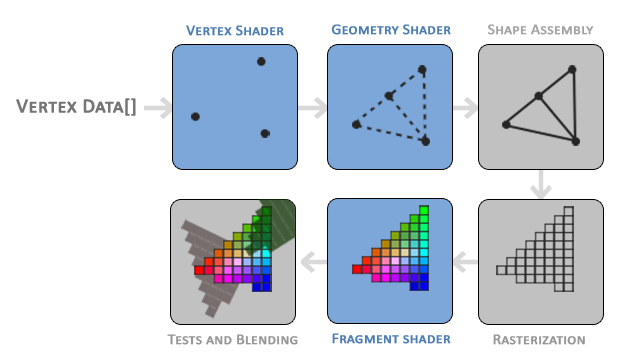
Credit: Joey de Vries,https://learnopengl.com/, CC BY 4.0
Meshes
Praxis: Visualizing meshes with ParaView
- File → Open… a mesh → Apply.
- Lighting/shading: set Representation = Surface.
Vector fields
Grids and unstructured meshes
- What is it? A vector (ux,uy,uz) per location; often paired with scalars (pressure, temperature).
- Acquire (by domain): CFD/FEA, climate/ocean models, MRI‑flow, EM fields.
- Used for: Flow direction/speed, vortices, transport, streamline topology.
- Stored as:
- Structured grids: VTI/NetCDF/XDMF+HDF5; rectilinear or curvilinear coordinates.
- Unstructured: VTU/VTK with per‑point or per‑cell vector arrays.
Vector fields
Grids and unstructured meshes
- Visualized with:
- Glyphs (arrows/cones) scaled by magnitude.
- Streamlines (steady) or pathlines/particle tracers (time‑varying).
Vector fields
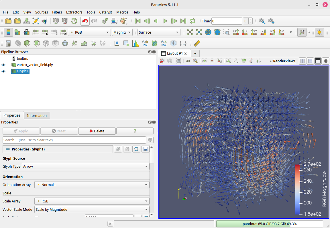
Praxis: Visualizing vector fields with ParaView
File → Open… a VTK/VTU/VTI/XDMF/NetCDF file with vectors → Apply.
Glyphs: Filters → Glyph.
- Vectors = your vector array (e.g., Velocity).
- Scale by = vector magnitude; set a sensible Scale Factor.
- Pick Glyph Type = Arrow (or Cone) → Apply.
It’s your turn!
- open Napari to look at 3D Pixel data
- open Paraview to look at Meshes, Point Clouds, and Vector Fields